Unit 9. Simple Linear Regression

Leyre Castro; J Toby Mordkoff

Unit 9. Simple Linear Regression

Leyre Castro and J Toby Mordkoff

Summary. This unit further explores the relationship between two variables with linear regression analysis. In a simple linear regression, we examine whether a linear relationship can be established between one predictor (or explanatory) variable and one outcome (or response) variable, such as when you want to see if time socializing can predict life satisfaction. Linear regression is a widely-used statistical analysis, and the foundation for more advanced statistical techniques.

Prerequisite Units

Unit 6. Brief Introduction to Statistical Significance

Unit 7. Correlational Measures

Linear Regression Concept

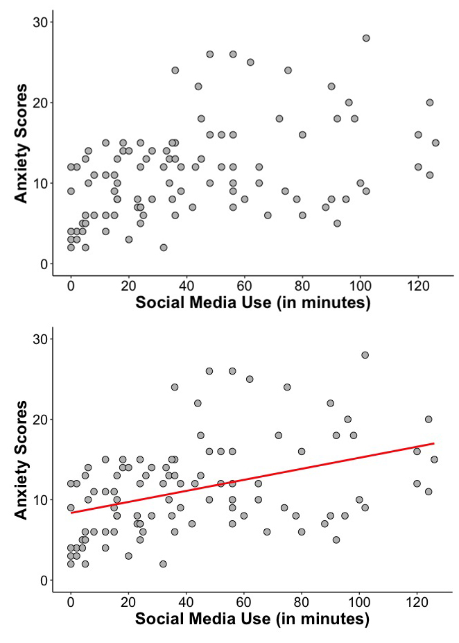
Imagine that we examine the relationship between social media use and anxiety in adolescents and, when analyzing the data, we obtain an r of 0.40, indicating a positive correlation between social media use and anxiety. The data points in the scatterplot on the top of Figure 9.1 illustrate this positive relationship. The relationship is even clearer and faster to grasp when you see the line included on the plot on the bottom. This line summarizes the relationship among all the data points, and it is called regression line. This line is the best-fitting line for predicting anxiety based on the amount of social media use. It also allows us to better understand the relationship between social media use and anxiety. We will see in this unit how to obtain this line, and what exactly means.

Figure 9.1. Scatterplots showing the relationship between social media use and anxiety scores. The scatterplots are exactly the same, except that the one on the bottom has the regression line added.

A linear regression analysis, as the name indicates, tries to capture a linear relationship between the variables included in the analysis. When conducting a correlational analysis, you do not have to think about the underlying nature of the relationship between the two variables; it doesn’t matter which of the two variables you call “X” and which you call “Y”. You will get the same correlation coefficient if you swap the roles of the two variables. However, the decision of which variable you call “X” and which variable you call “Y” does matter in regression, as you will get a different best-fitting line if you swap the two variables. That is, the line that best predicts Y from X is not the same as the line that predicts X from Y.

In the basic linear regression model, we are trying to predict, or trying to explain, a quantitative variable Y on the basis of a quantitative variable X. Thus:

The X variable in the relationship is typically named predictor or explanatory variable. This is the variable that may be responsible for the values on the outcome variable.
The Y variable in the relationship is typically named outcome or response or criterion variable. This is the variable that we are trying to predict/understand.

In this unit, we will focus on the case of one single predictor variable, that’s why this unit is called “simple linear regression.” But we can also have multiple possible predictors of an outcome; if that is the case, the analysis to conduct is called multiple linear regression. For now, let’s see how things work when we have one possible predictor of one outcome variable.

Linear Regression Equation

You may be interested in whether the amount of caffeine intake (predictor) before a run can predict or explain faster running times (outcome), or whether the amount of hours studying (predictor) can predict or explain better school grades (outcome). When you are doing a linear regression analysis, you model the outcome variable as a function of the predictor variable. For example, you can model school grades as a function of study hours. The formula to model this relationship looks like this:

$\begin{equation*} \hat{Y} = b_0 + b_1X \end{equation*}$

And this is the meaning of each of its elements:

$\hat{Y}$ (read as “Y-hat”) = the predicted value of the variable Y

$\ b_0$ = the intercept or value of the variable when the predictor variable X = 0

$\ b_1$ = the slope of the regression line or the amount of increase/decrease in Y for each increase/decrease in one unit of X

$\ X$ = the value of the predictor variable

When we conduct a study, the data from our two variables X and Y are represented by the points in the scatterplot, showing the different values of X and Y that we obtained. The line represents the $\hat{Y}$ values, that is, the predicted values of Y when we use the X and Y values that we measured in our sample to calculate the regression equation. Figure 9.2 shows a regression line depicting the relationship between number of study hours and grades, and where you can identify the intercept and the slope for the regression line.

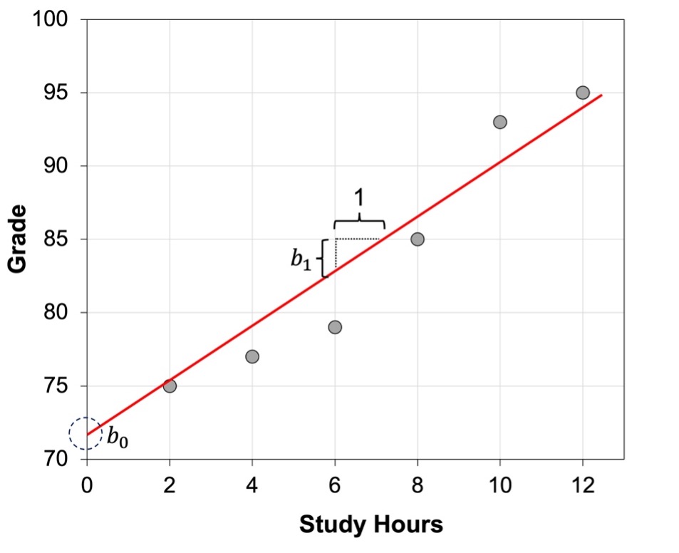
Figure 9.2. Regression line depicting the relationship between number of study hours and grades. For the sake of clarity, only 6 observations are included. Here, the intercept is equal to 72, and the slope is equal to approximately 2. You can check and see that, regardless of where you measure the slope, its value is always the same.

We have defined the intercept as the value of $\hat{Y}$ when X equals zero. Note that this value may be meaningful in some situations but not in others, depending on whether or not having a zero value for X has meaning and whether that zero value is very near or within the range of values of X that we used to estimate the intercept. Analyzing the relationship between the number of hours studying and grades, the intercept would be the grade obtained when the number of study hours is equal to 0. Here, the intercept tells us the expected grade in the absence of any time studying. That’s helpful to know. But let’s say, for example, that we are examining the relationship between weight in pounds (variable X) and body image satisfaction (variable Y). The intercept will be the score in our body image satisfaction scale when weight is equal to 0. Whatever the value of the intercept may be in this case, it is meaningless, given that it is impossible that someone weighs 0 pounds. Thus, you need to pay attention to the possible values of X to decide whether the value of the intercept is telling you something meaningful. Also, make sure that you look carefully at the x-axis scale. If the x-axis does not start at zero, the intercept value is not depicted; that is, the value of Y at the point in which the regression line touches the y-axis is not the intercept if the x-axis does not start at zero.

The critical term in the regression equation is b₁ or the slope. We have defined the slope as the amount of increase or decrease in the value of the variable Y for a one-unit increase or decrease in the variable X. Therefore, the slope is a measure of the predicted rate of change in Y. Let’s say that the slope in the linear regression with number of study hours and grades is equal to 2.5. That would mean that for each additional hour of study, grade is expected to increase 2.5 points. And, because the equation is modeling a linear relationship, this increase in 2.5 points will happen with one-unit increase at any point within our range of X values; that is, when the number of study hours increase from 3 to 4, or when they increase from 7 to 8, in both cases, the predicted grade will increase in 2.5 points.

The different meanings of β

The letter b is used to represent a sample estimate of the β coefficient in the population. Thus b₀ is the sample estimate of β₀, and b₁ is the sample estimate of β₁. As we mentioned in Unit 1, for sample statistics we typically use Roman letters, whereas for the corresponding population parameters we use Greek letters. However, be aware that β is also used to refer to the standardized regression coefficient, a sample statistic. Standardized data or coefficients are those that have been transformed so as to have a mean of zero and a standard deviation of one. So, when you encounter the symbol β, make sure you know to what it refers.

How to Find the Values for the Intercept and the Slope

The statistical procedure to determine the best-fitting straight line connecting two variables is called regression. The question now is to determine what we mean by the “best-fitting” line. It is the line that minimizes the distance to our data points or, in different words, the one that minimizes the error between the values that we obtained in our study and the values predicted by the regression model. Visually, it is the line that minimizes the vertical distances from each of the individual points to the regression line. The distance or error between each predicted value and the actual value observed in the data is easy to calculate:

$\begin{equation*} \ error = \ Y - \hat{Y} \end{equation*}$

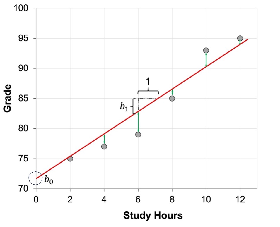
This “error” or residual, as is also typically called, is not an error in the sense of a mistake. It tries to capture variations in the outcome variable that may occur due to unpredicted or unknown factors. If the observed data point lies above the line, the error is positive, and the line underestimates the actual data value for Y. If the observed data point lies below the line, the error is negative, and the line overestimates that actual data value for Y (see error for each data point in green in Figure 9.3). For example, in Figure 9.3, our regression model overestimates the grade when the number of study hours are 6, whereas it underestimates the grade when the number of study hours are 10.

Because some data points are above the line and some are below the line, some error values will be positive while others will be negative, so that the sum of all the errors will be zero. Because it is not possible to conduct meaningful calculations with zero values, we need to calculate the sum of all the squared errors. The result will be a measure of overall or total squared error between the data and the line:

$\ total \medspace squared \medspace error = \sum {(Y- \hat {Y})^2}$

So, the best-fitting line will be the one that has the smallest total squared error or the smallest sum of squared residuals. In addition, the residuals or error terms are also very useful for checking the linear regression model assumptions, as we shall see below.

Getting back to our calculations, we know that our regression equation will be the one that minimizes the total squared error. So, how do we find the specific values of b₀ and b₁ that generate the best-fitting line?

We start calculating b₁, the slope:

$\begin{equation*}\ b_1 = r (\frac {s_y} {s_x}) \end{equation*}$

where $\s_y$ = the standard deviation of the Y values and $\s_x$ = the standard deviation of the X values (that you learned to calculate in Unit 3) and r is the correlation coefficient between X and Y (that you learned to calculate in Unit 7).

Once we have found the value for the slope, it is easy to calculate the intercept:

$\begin{equation*}\ b_0 = \bar{Y} - b_1 \bar{X} \end{equation*}$

Practice

Any statistical software will make these calculations for you. But, before learning how to do it with R or Excel, let’s find the intercept and the slope of a regression equation for the small dataset containing the number of study hours before an exam and the grade obtained in that exam, for 15 participants, that we used previously in Unit 3 and Unit 7. These are the data:

Participant	Hours	Grade
P1	8	78
P2	11	80
P3	16	89
P4	14	85
P5	12	84
P6	15	86
P7	18	95
P8	20	96
P9	10	83
P10	9	81
P11	16	93
P12	17	92
P13	13	84
P14	12	83
P15	14	88

As you can tell from the formulas above, we need to know the mean and the standard deviation for each of the variables (see Unit 3). From our calculations in Unit 3, we know that the mean number of hours ( $\bar{X}$ ) is 13.66, and the mean grade obtained in the exam ( $\bar{Y}$ ) is 86.46. We also know that the standard deviation for hours ( $\ s_x$ ) is 3.42, and the standard deviation for grade ( $\ s_y$ ) is 5.53. In addition, from our calculations in Unit 7 we know that r for the relationship between study hours and grade is 0.95. So, let’s calculate first the slope for our regression line:

$\ b_1$ = 0.95 * (5.53 / 3.42)

that is:

$\ b_1$ = 1.54

Once we have $\ b_1$ , we calculate the intercept:

$\ b_0$ = 86.46 (the mean grade in the exam) – 1.54 * 13.66 (the mean number of study hours)

that is:

$\ b_0$ = 65.47

So, our regression equation is:

$\begin{equation*}\hat{Y} = 65.47 + 1.54*X \end{equation*}$

This means that the expected grade of someone who studies 0 hours will be 65.47, and that for each additional hour of study, a student is expected to increase their grade in 1.54 points.

Linear Regression as a Tool to Predict Individual Outcomes

The regression equation is useful to make predictions about the expected value of the outcome variable Y given some specific value of the predictor variable X. Following with our example, if a student has studied for 15 hours, their predicted grade will be:

$\hat{Y}$ = 65.47 + 1.54*15

that is:

$\hat{Y}$ = 88.57

Of course, this prediction will not be perfect. As you have seen in Figure 9.3, our data points do not fit perfectly on the line. Normally, there is some error between the actual data points and the data predicted by the regression model. The closer the data points are to the line, the smaller the error is.

In addition, be aware that we can only calculate the $\hat{Y}$ value for values of X that are within the range of values that we included in the calculation of your regression model (that is, we can interpolate). We cannot know if values that are smaller or larger than our range of X values will display the same relationship. So, we cannot make predictions for X values outside the range of X values that we have (that is, we cannot extrapolate).

Linear Regression as an Explanatory Tool

Note that, despite the possibility of making predictions, most of the times that we use regression in psychological research we are not interested in making actual predictions for specific cases. We typically are more concerned with finding general principles rather than making individual predictions. We want to know if studying for a longer amount of time will lead to have better grades (although you probably already know this) or we want to know if social media use leads to increased anxiety in adolescents. The linear regression analysis provides us with an estimate of the magnitude of the impact of a change in one variable on another. This way, we can better understand the overall relationship.

Linear regression as a statistical tool in both correlational and experimental research

Linear regression is a statistical technique that is independent of the design of your study. That is, whether your study is correlational or experimental, if you have two numerical variables, you could use a linear regression analysis. You need to be aware that, as mentioned at different points in this book, if the study is correlational, you cannot make causal statements.

Assumptions

In order to conduct a linear regression analysis, our data should meet certain assumptions. If one or more of these assumptions are violated, then the results of our linear regression may be unreliable or even misleading. These are the four assumptions:

1) The relationship between the variables is linear

The values of the outcome variable can be expressed as a linear function of the predictor variable. The easiest way to find if this assumption is met is to examine the scatterplot with the data from the two variables, and see whether or not the data points fall along a straight line.

2) Observations are independent

The observations should be independent of one another and, therefore, the errors should also be independent. That is, the error (the distance from the obtained Y to the $\hat{Y}$ predicted by the model) for one data point should not be predictable from knowledge of the error for another data point. Knowing whether this assumption is met requires knowledge of the study design, method, and procedure. If the linear regression model is not adequate, this does not mean that the data cannot be analyzed; rather, other analyses are required to take into account the dependence among the data observations.

3) Constant variance at every value of X

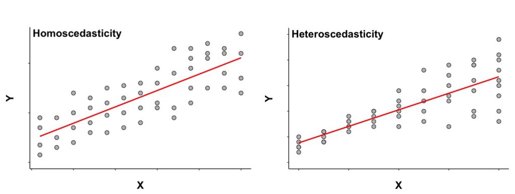
Another assumption of linear regression is that the residuals should have constant variance at every value of the variable X. In other words, variation of the observations around the regression line are constant. This is known as homoscedasticity. You can see on the scatterplot on the left side of Figure 9.4 that the average distance between the data points above and below the line is quite similar regardless of the value of the X variable. That’s what homoscedasticity means. However, on the scatterplot on the right, you can see the data points close to the line for the smaller values of X, so that variance is small at these values; but, as the value of X increases, values of Y vary a lot, so some data points are close to the line but others are more spread out. In this case, the constant variance assumption is not met, and we say that the data show heteroscedasticity.

Figure 9.4. On the left, a scatterplot showing homoscedasticity: that is, the variance is similar at all levels of the variable X. On the right, a scatterplot showing heteroscedasticity; in this case, the variance of the observations for the lower values of the variable X is much smaller (the data points are tighter and closer to the line) than the variance for the higher values of the variable X.

When heteroscedasticity (that is, the variance is not constant but varies depending on the value of the predictor variable) occurs, the results of the analysis become less reliable because the underlying statistical procedures assume that homoscedasticity is true. Alternatives methods must be used when the data as heteroscedasticity is present.

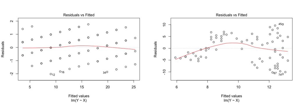
When we have a linear regression model with just one predictor, it may be possible to see whether or not the constant variance assumption is met just looking at the scatterplot of X and Y. However, this is not so easy when we have multiple predictors, that is, when we are conducting a multiple linear regression. So, in general, in order to evaluate whether this assumption is met, once you fit the regression line to a set of data, you can generate a scatterplot that shows the fitted values of the model against the residuals of those fitted values. This plot is called a residual by fit plot or residual by predicted plot or, simply, residuals plot.

In a residual plot, the x-axis depicts the predicted or fitted Y values ( $\hat{Y}$ s), whereas the y-axis depicts the residuals or errors, as you can see in Figure 9.5. If the assumption of constant variance is met, the residuals will be randomly scattered around the center line of zero, with no obvious pattern; that is, the residuals will look like an unstructured cloud of points, with a mean around zero. If you see some different pattern, heteroscedasticity is present.

Figure 9.5. On the left, a residuals plot where the errors are evenly distributed without showing any pattern, an indication of homoscedasticity. On the right, a residuals plot where the errors show different patterns depending on the fitted values of Y, a sign heteroscedasticity.

4) Error or residuals are normally distributed

The distribution of the outcome variable for each value of the predictor variable should be normal; in other words, the error or residuals are normally distributed. The same as with the assumption of constant variance, it may be possible to visually identify whether this assumption is met by looking at the scatterplot of X and Y. In Figure 9.4 above, for example, you can see that in both scatterplots the distance between the actual values of Y and the predicted value of Y is quite evenly distributed for each value of the variable X, suggesting therefore a normal distribution of the errors on each value of X. So, note that, even if the constant variance assumption is not met, the residuals can still be normally distributed.

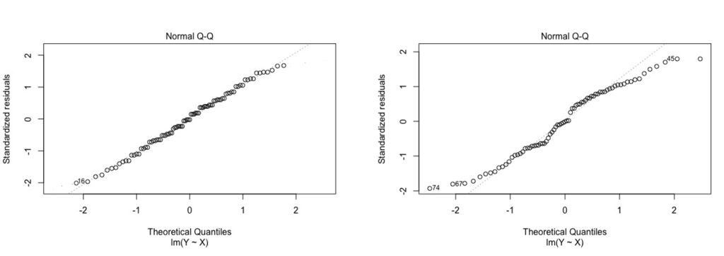
A normal quantile or quantile-quantile or Q-Q plot of all of the residuals is a good way to check this assumption. In a Q-Q plot, the y-axis depicts the ordered, observed, standardized, residuals. On the x-axis, the ordered theoretical residuals; that is, the expected residuals if the errors are normally distributed (see Figure 9.6). If the points on the plot form a fairly straight diagonal line, then the normality assumption is met.

Figure 9.6. On the left, a Q-Q plot showing a normal distribution of the residuals, so that this assumption is met. On the right, a Q-Q plot showing a non-normal distribution of the residuals, so that this assumption is not met.

It is important to check that your data meet these four assumptions. But you should also know that regression is reasonably robust to the equal variance assumption. Moderate degrees of violation will not be problematic. Regression is also quite robust to the normality assumption. So, in reality, you only need to worry about severe violations.

License

Icon for the Creative Commons Attribution-NonCommercial-ShareAlike 4.0 International License

Data Analysis in the Psychological Sciences: A Practical, Applied, Multimedia Approach Copyright © 2023 by Leyre Castro & J Toby Mordkoff is licensed under a Creative Commons Attribution-NonCommercial-ShareAlike 4.0 International License, except where otherwise noted.

Linear Regression Concept

Linear Regression Equation

How to Find the Values for the Intercept and the Slope

Linear Regression as a Tool to Predict Individual Outcomes

Linear Regression as an Explanatory Tool

Assumptions

1) The relationship between the variables is linear

2) Observations are independent

3) Constant variance at every value of X

4) Error or residuals are normally distributed

License

Share This Book