Summary.  This unit introduces some of the basic concepts of statistics as they apply to psychological research. These concepts include data and variables, populations and samples, and the distinction between descriptive and inferential statistics.

Statistics to Better Understand the World

We live in a data-driven world.  We use data in science, sports, business, politics, public health; we collect data from surveys, polls, and ratings; and we measure how much we walk, drive, eat and sleep.  We want to know how things are now and how to guide our future actions.  Before making a decision, we gather information.  Frequently, this means gathering numbers: fuel efficiency, engine capacity, acceleration rate, and market price if we are planning to buy a car; admission rate and likelihood of having a job after graduating if we are deciding what college to attend; or how many miles we run and changes in our heart rate if we are trying to improve our physical fitness.  In summary, we are constantly measuring our world, because we want to understand it and make the best decisions.

But collecting numbers and measurements is not enough.  We need to try to make sense of all that information, which can sometimes be overwhelming.  We don’t want to draw false conclusions or make poor decisions.  Thus, careful analysis of the data is necessary, to be able to comprehend their meaning, to be able to find patterns, to evaluate actions and behaviors, to uncover trends and estimate the future.  Statistics will help us to see through the forest of data more clearly and achieve these goals.

We need to understand and make sense of the data regardless of our biases, wishes, and preferences.  That is, we need to be objective and see what the data are telling us, regardless of what we might want to see.  That’s why we need statistics.  Nonetheless, statistics may not give you a simple, single answer.  But they will help you condense information so that it’s easier to manage and understand.  Statistics may not capture the full richness, nuances, color, and texture of the world, but they are the most powerful tool that we have to objectively understand what we are and what happens around us.

Psychology as an Empirical Science

Psychological science aims to understand human (and animal, in general) behavior from an empirical point of view.  That is, we use objective observations and measurements to test our theories and hypotheses about how humans behave.  But psychological science will only be as good as the quality of the observations that we use are.

Anecdotes or intuition or “common sense” may seem to serve us sometimes in our daily lives.  But they are subject to all kind of biases.  That type of information is inadequate to build a solid and trustable discipline.  We need to acquire information using a scientific methodology.

When we do science, it is not about our opinions or wishes.  We try to understand events and behaviors by finding patterns in empirical observations and carefully analyzing how those observations are related.  Yes, we have opinions, and beliefs, and desires, and intuitions.  But none of these can help explain reality.

Science can help us to understand and explain events and behaviors.  We develop hypotheses and we conduct detailed empirical observations to test those hypotheses.  These detailed observations are our data.  Careful statistical analysis of our data will allow us to support or reject our hypotheses.  This knowledge will allow us in turn to build theories to understand events and behaviors.  These theories will also allow us to make new predictions –to generate new hypotheses that will further advance our comprehension of those events and behaviors.

Statistics may sometimes give us an imperfect representation of reality.  We measure different people at different times in different places, so it may be sometimes difficult to extract conclusions that can apply to absolutely everybody.  That’s why we need to learn not only to conduct our statistical analysis, but to critique and evaluate others’.  Being objective while keeping a critical eye will help us to make the best of our statistical understanding of our world.

Data and Variables

The word data (which is technically plural) refers to any organized set of observations.  An observation is a value –which can be a number or a label, such as “red”– that tells you something about something.  In some cases, an observation specifies the value of a person on some dimension, such as their age or their current level of depression.  In other cases, an observation can refer to the behavior of a person, such as what they said when asked a particular question, whether they answered a question correctly, or how quickly they responded on a trial in a laboratory experiment.  It does not matter if the observation was collected by watching the person, talking to them, or having a computer measure something like a response time; whenever you get a new piece of information, the value that you got is an observation.

Each observation specifies a value on a dimension, such as age, favorite color, level of depression, correctness, or speed of response.  In statistical parlance, these dimensions are referred to as variables.  A variable is anything that has more than one possible value.

The values of some variables differ mathematically because they tell you the amount of something.  These variables are called quantitative, because they specify a quantity; examples of quantitative variables include age and response time.  Most quantitative variables also have units.  The units make it clear what the numbers refer to (i.e., how much of what).  Note that it is quite possible to have two variables that refer to the same general concept, such as time, but use very different units; age vs response time is a good example.  For age, we usually use years as the unit, but we could use months or even weeks if we are concerned with infants’ ages.  For response time, we usually use milliseconds (i.e., thousandths of a second), but we could use minutes if we are asking people to wait in a self-control task.  It is crucial to keep track of the units.  It would (probably) be very wrong to say that a person took 350 years to make a response or that they were only 19 milliseconds old.

Other variables take on values that differ in ways that are categorical, instead of numerical, in which case the variable is called qualitative, since it specifies a quality.  Examples of qualitative variables include favorite food or TV show, ethnic group, and handedness.  Some qualitative variables require a label or something like units.  It’s not enough to know that the value for a person is “strawberry shortcake”; you need to know if this refers to the food or to the cartoon character.  The key is to always think of an observation as specifying the value of something on some dimension.  If it isn’t obvious to what dimension the value refers, make sure to include it somewhere.

There is one other type of variable, which can be thought of as being somewhere between quantitative and qualitative.  These are called ordinal variables.  An ordinal variable specifies a position in a sequence or list, and uses a number to do this, such as 1st, 2nd, 3rd, etc., but these numbers do not refer to an amount of something (so they’re not quantities).  The best example of this in psychology is birth order, which is known to be very important to a variety of things, from attachment (to the primary caregivers) to performance in school.  Assuming a family with three children, none of whom are twins, one child is 1st, another is 2nd, and the last is 3rd.  This might seem numerical, but it is not either a ratio or interval scale (see previous box).  The 2nd-born is not “twice” the 1st-born in any meaningful way (so it is not a ratio scale), and the gap in time between the 1st and 2nd child does not have to be the same as the gap between 2nd and 3rd (so it isn’t an interval scale).  In general, it would be inaccurate to take 1st, 2nd, 3rd, etc, as specifying amounts or quantities in the usual sense.  But they are more than just categories, because they have an order, which allows us to conduct certain analyses that don’t work for qualitative categories, such a favorite color or handedness.  Therefore, we keep ordinal variables separate from the other two types.

The quantitative vs. qualitative vs. ordinal distinction is inherent to the variable and does not depend on how the variable is being used.  Another way that variables differ, however, does depend on the role that the variable is playing.  On one side, there are independent or manipulated variables.  These are properties, characteristics, or qualities that are entirely determined or set by the experimenter.  For example, in an experiment concerning the effects of sleep deprivation on something like mood, the number of hours of sleep –if it is controlled by the experimenter– is an independent variable (IV).  On the other side, there are dependent or measured variables.  These are properties, characteristics, or qualities that are observed as they occur.  In the case of the sleep-deprivation experiment, “grumpiness” on a ten-point scale might be the dependent variable (DV).

Note that IV and DV are not automatic labels for a given property, characteristic, or quality.  Some variables can be used as either an IV or DV, depending on the context.  For example, hours of sleep can be the IV in a sleep-deprivation experiment, where the amount of sleep is controlled and restricted by the experimenter, or it can be a DV in a study of depression or anxiety, where the participant is asked how much sleep they have been getting in order to take this information into account to better evaluate depression or anxiety.  It is crucial that you correctly identify how a given variable is being used in a given line of research.  The best way to do this is to remember the alternative names for IV and DV and ask: was this variable manipulated or was it measured by the researcher?

There is also what appears to be a third class of variables that is somewhere between an IV and DV.  These subject variables (SVs) are properties, characteristics, or qualities that vary across research subjects, but are relatively stable within subjects (across time) and/or are extremely difficult or impossible to manipulate.  Some classic examples are handedness, ethnicity, and sex and/or gender, but “higher-order” examples also exist, such as socio-economic status.  The value of an SV is measured, not manipulated, which makes them like a DV, but they are sometimes treated as if they had been manipulated, which makes them a bit like IVs.  In other analyses, SVs play a very special role –known as a covariate– that is different from both an IV or DV.

The last way in which variables differ has no agreed-upon label; we shall refer to it as kind.  The first kind of data is raw; these are single observations as they were originally recorded.  This can be the response time on one trial in an experiment or the answer to a single item on a questionnaire.  This might be surprising, but this kind of data is not used very often in research.

The second kind of data are summary scores; these are created from multiple observations of the same thing under the same set of conditions.  The best example of this is how response time is usually measured.  It is very rare to run just one trial in each condition of a response-time experiment.  Usually, there’s 20 or more trials in each condition and the average time across all (correct) trials is kept for analysis.  In other words, the 20 or more raw pieces of data are converted to one summary score.  (The reason that this is done, as you will see later, is that summary scores are much less “noisy” than raw scores, which increases the power of the statistical analysis.)

The last kind of data are condensed or composite or scale scores (any of these labels is fine).  These are created from multiple observation of different things.  Examples of this include the standard measures of depression and anxiety.  For both of these, the person is asked many different questions, from which a single (numerical) value can be calculated.  This is similar to a summary score in that many raw scores are somehow combined; the difference is that a summary score is based on many measures of the same thing, whereas a condensed score is based on many measures of different things.  The reason that condensed scores are used is that it is often impossible to measure all aspects of a psychological construct, such as depression or anxiety, in just one question; to get all of the aspects of the construct of interest, many questions are needed.

The statistical procedures that we will be using make no distinction between the three kinds of data.  Put bluntly, the statistical procedures do not care about the kind of data.  It is also quite possible for different kinds of data to be mixed in a given analysis.  For example, personality might be defined in terms of five [condensed] scores (as is done for the Big Five model of personality) and then used in combination with [raw] gender and [summarized] mean number of miles driven per day.  Why would one do this?  Maybe in an attempt to understand what causes road-rage.

Although the kinds of data being used may have no effect on the method of analysis, they can have profound effects on interpretation.  For example, because most information-processing experiments use the mean of response time across many trials (as opposed to the individual, raw values from each of the trials), the proper conclusions from these experiments concern “average” performance and not specific acts.  When a difference is observed between two condition means in a typical response-time experiment, the correct conclusion is that “average” performance in one of the conditions is better than in the other, not that performance is “always” or even “usually” better.

Populations and Samples

Warning: the technical meaning of the word population is very different from the everyday meaning.

Recall from earlier that an observation tells you something about something.  Taking the above discussion of variables into account, we can now update this to say that an observation tells you the value of a variable.  But who or what has this particular value of this particular variable?  That is the domain of population and samples.

In the context of research, the word population refers to the set of all creatures, objects, or events that have values of the variable(s) that you are investigating.  If you’re interested in depression as measured by a standard questionnaire, then the population will probably be all living people.  If you’re doing research on the neural connections between two different parts of the brain using drugs or lesions, then your population might be all white laboratory rats, instead of all people.  In both of these examples, the word population refers to every creature to which your results might apply.  This isn’t very different from the everyday use of the word population.

In contrast, if you are doing research on word recognition, then your population might be the set of all words in the language you’re using.  The words that you use all have values of variables.  Each word is from a part-of-speech (i.e., noun, verb, adjective, etc., which is a qualitative variable); each word also has a number of letters and a number of syllables (which are both discrete quantitative variables).  So, the set of all words in a language is also a population.

Similarly, if you are studying road-rage by doing field observations, then your population might be something like intersections.  These also have values on variables, such as number of lanes or length of red-light.  Finally, in some (rare) cases, the population can be the set of all events of a certain type, such as all hurricanes in the last 100 years.  These also have values on variables, such as maximum wind-speed or amount of rainfall.

One thing that all populations have in common is that it is difficult to impossible to include every member or instance in your research.  This is where samples come in.  A sample is a subset of a population – it is the subset that was actually included in your experiment or correlational study.  In the ideal case, your sample will be “representative” of the whole population.  (A sample is said to be representative when all members of the population have an equal chance of being included.)  In some situations, this might not be possible.  This brings us to another distinction.  The term target population refers to the set of all people, objects, or events in which you are interested and/or want to make statements about.  The term sampling population refers to the set of all people, objects, or events that have a chance of being included in your sample.  In the ideal case, the sampling population will be the same as the target population.  In actual research, they are often different.

The typical relationship between the target population, sampling population, and sample is shown in the picture to the right.  Note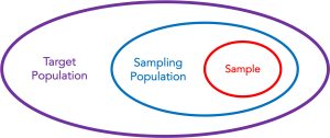 that it is possible (in a few, rare situations) for the sampling population to be as large as and, therefore, the same as the target population, but the sample is always a (relatively small) subset of the sampling population.  This is what makes it a sample.

What allows us to draw conclusions about the entire target population from just the data in a sample?  As suggested by the previous picture, this is a two-step process.  The first step goes from the sample to the sampling population (e.g., from the people who actually signed up for your experiment to all students in the Elementary Psychology Subject Pool).  This is achieved by a certain type of statistics, which will be defined next and will be described in more detail in subsequent units.  The second step goes from the sampling population to the target population (e.g., from all students in the Elementary Psychology Subject Pool to all people who have the variables that you investigate).  This requires something called external validity, which is not a statistical issue.

Standard Symbols

The distinction between samples and populations is very important, as is the difference between descriptive statistics –which are summaries of samples– and inferential statistics –which provide estimations of populations.  To help keep these separate, we use different symbols for each.

For samples and descriptive statistics, we use Roman letters.  For example, we use the letter n for the number of observations.  We use the letter M (or m or mn) for the mean of the sample, which is the most popular way to get an average value of a quantitative variable.  We use the letter r for the correlation between two quantitative variables in a sample.

For populations, we use Greek letters, instead.  The mean of the population –which is what we are usually trying to estimate– uses μ (mu, pronounced “mee-you” mashed together in one syllable) which is the Greek version of (lower-case) m.  Likewise, the value of a correlation in the (entire) population uses ρ (rho, pronounced “row”), which is a Greek (lower-case) r.

Certain upper-case Greek letters are used for mathematical operations.  For example, if you want to say “add up the values of all of these numbers,” you can do this by using ∑ (“sig-muh”), which is an upper-case S, short for the word sum.  Similarly, if you want to say “multiply all of these values together,” you can use Π (“pie”), which is an upper-case P, short for the word product.

Descriptive vs Inferential Statistics

Assume that you are interested in knowing the average hours of sleep that people are getting per night.  As discussed above, you are not going to learn this by measuring the hours of sleep for every living person; you aren’t even going to measure this for every student in the Elementary Psychology Subject Pool.  Instead, you will probably take a relatively small sample of students (e.g., 100 people), ask each of them how many hours of sleep they usually get, and then use these data to calculate an estimate of the average for everybody.

The process outlined above is best thought of as having three phases or steps: (1) collect the sample, (2) summarize the data in the sample, and then (3) use the summarized data to make an estimate of the entire population.  The issues related to collecting the sample, such as how one ensures that the sample is representative, will not be discussed in these modules; they are not part of statistics.  The second step is referred to as descriptive statistics and will be the focus of the units in this textbook.  The third step is called inferential statistics and will covered in future materials.

The purpose and value of descriptive statistics is that they organize and summarize large sets of data.  They allow researchers to communicate quickly.  Instead of having to list every value of every variable for every participant, the researcher can report a few numbers or draw a few pictures that capture most of the important information.  Because they are summaries, they leave out some detail; but, because they are summaries, they can be very brief and efficient.

The main limitation of descriptive statistics is that they only describe (or make statements about) the actual sample.  In other words, descriptive statistics never go beyond what we know for sure.

In contrast, inferential statistics allow us to go beyond the data in hand and calculate estimates of (or make statements about) the population from which the sample was taken.  Although this is the ultimate goal of the research, it’s important to note in advance that inferential statistics aren’t guaranteed to be 100% accurate; they are educated guesses or estimations, not deductive conclusions.  Whenever you use an inferential statistic, you need to keep track of how wrong you might be.