Appendix 1 – Statistical Analysis of Data

Russell Larsen; Mouna Maalouf

Appendix 1 – Statistical Analysis of Data

Whenever a numerical result is reported, you should ask: Does the number really come close to the “true value?” This is not an easy question, but it is one that deserves some thought. This appendix provides you with some of the vocabulary and techniques that can be used to think about this question. You may not necessarily use everything in this appendix, but you will when you take more advanced courses that use experimentally measured values.

During this semester, you will be using several pieces of equipment to make measurements: thermometer for temperature measurements, burets for volume measurements, and balances for mass measurements, to name a few. The choice of equipment will influence the results that you obtain. This is because each piece of equipment differs not only in their basic functions but also in their sensitivity (the minimum amount that can reliably be measured) and capacity (the maximum amount that can reliably be measured). For example, if you were asked to determine the mass of a penny, a bathroom scale would be an inappropriate measuring device since it is not sensitive enough to measure such a small mass; an analytical balance would be a more appropriate device. On the other hand, if you were asked to determine the weight of your lab partner, a bathroom scale would be appropriate since it has sufficient sensitivity and capacity for this task. In contrast, the analytical balance lacks the capacity for such a large weight. Part of laboratory science is to determine which device is most suitable for making a specific measurement. You must decide on the sensitivity and capacity required for the measurement and which device fulfills this requirement most easily (and often at the lowest price).

Further, each device used will also have an associated uncertainty (also called error), which is often related to the sensitivity of the device (e.g. you cannot measure an ant on a bathroom scale). Measurements are rarely exact; associated with each measurement is an uncertainty or error. It is useful to distinguish between two types of error encountered in scientific experiments: systematic errors and random errors. (A third type, illegitimate error, such as spilling or misreading the instrument, is assumed to be eliminated by careful laboratory technique.) Systematic errors (also known as determinate errors) are errors with potentially definable causes that affect the measurement in a defined direction, i.e. they skew the data either higher or lower than the “true value”. (The quotation marks remind us that in general the “true value” is only an ideal value that is unknown.) Systematic errors affect the accuracy of the resulting measurements. The accuracy of the experimental results is the difference between the measured results and the “true value”. For example, at the doctor’s office where the scales are well calibrated, a person is measured to weigh 160 lbs., but at home on a bathroom scale that same person might consistently be measured as 155 lbs. In this case, the bathroom scale is not accurate and has a systematic error of –5 lbs. (Notice the negative sign that indicates that the scale read less than the “true value.”)

The second type of error, random error (also known as indeterminate error), is due to the inherent difficulty in repeating identical measurement procedures. When repetitive measurements of apparently identical experiments are made, random errors introduce scatter into the data relative to the “true value.” On average as many “too high” readings as “too low” readings are obtained relative to the true value. The amount of scatter in any set of data is referred to as the precision of the measurement.

The classic analogy to distinguish between precision and accuracy is illustrated by the set of dart boards given below.

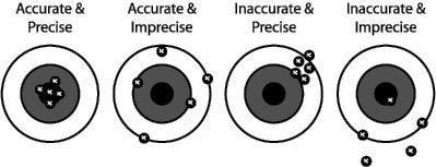
If the bull’s eye represents the “true value” and each throw indicates one datum, the distances between the data and the bull’s eye represent the errors. Each dart board represents a different combination of accuracy and precision.

Although this gives a qualitative picture of the concepts, a quantitative measure of the uncertainty (error) is necessary in order for these concepts to be useful for numerical data analysis. For data subject only to random error (it is assumed that systematic error has been eliminated by proper calibration), an experimental result is often reported as the mean value (or average) of the data, and the precision of the result is indicated by showing the calculated standard deviation of the data. When reporting such a result, it is also important to include the number of measurements that were used to calculate the mean so that the accuracy can be statistically judged.

The first step in such a statistical treatment of the data is to find the mean (also called the average value). The mean is usually given by the symbol, $\displaystyle \bar{\textbf{X}}$ (said x bar), and is found by taking the sum of the data points and dividing by the number of individual results. Mathematically, the mean is defined as,

$\displaystyle \bar{x}=\frac{\sum_{i=1}^{i=n}{x_i}}{n}=\frac{x_1+x_2+\dots+x_n}{n}$

where $\displaystyle \bar{\textbf{X}}$ is the mean and the sum is from the first data point, $\displaystyle {{x}_{1}}$ , to the $\displaystyle {{n}^{{th}}}$ data point $\displaystyle {{x}_{n}}$ . The mean represents the best estimate of the “true value” based on the experimental data. “True value” is often given the symbol $\displaystyle \mu$ ; $\displaystyle {{\mu }_{{true}}}$ will be used here. [In Excel®, the mean is found using the function, =AVERAGE(A3:A6), where A3:A6 represents the data present in the A column in rows 3-6.]

The second step in a statistical treatment of the data is to obtain the precision of the data (the scatter). This is done by calculating the standard deviation of the data. To find the standard deviation, the difference between the mean and each experimental value is taken and the resultant is then squared; the sum of each of the squares is then taken and divided by the number of data points minus one; finally the square root is taken. Mathematically, the standard deviation is defined as,

$\displaystyle s=\sqrt{\frac{\sum_{i=1}^{i=n}{(x_i-\bar{x})^2}}{n-1}}=\sqrt{\frac{\left(x_1-\bar{x}\right)^2+\left(x_2-\bar{x}\right)^2+\dots+\left(x_n-\bar{x}\right)^2}{n-1}}$

where s is the standard deviation. Some authors find it useful to distinguish between standard deviations that are obtained from experimental data and the “true” or ideal standard deviation that would be obtained after an infinite number of measurements. In the former case, the standard deviation is usually designated by the letter ‘s’ and in the latter by the Greek letter ‘ $\displaystyle \sigma$ ’ (sigma). However, this convention is not universally applied, and in fact, it is common to find $\displaystyle \sigma$ used without distinction. [In Excel®, the standard deviation is found using the function, =STDEV.S(A3:A6), where A3:A6 represents the data present in the A column in rows 3-6.]

The denominator, (n-1), of the standard deviation expression is known as the degrees of freedom. When the “true value” is not known a priori, this term has a value of n-1 since it takes one degree of freedom to determine the mean. The mean is the experimental best estimate of the “true value”.

Now consider an example of statistical analysis of some sample data. Suppose a titration of a weak acid with a strong base is carried out five times with the following results:

Experiment number I	Volume of $\displaystyle NaOH$ used in mL	$\displaystyle \left( {{{x}_{i}}-\bar{x}} \right)$ in mL	$\displaystyle {{\left( {{{x}_{i}}-\bar{x}} \right)}^{2}}$ in mL²
1	12.05	0.012	0.00014
2	12.03	0.008	0.00006
3	12.06	0.022	0.00048
4	12.02	0.018	0.00032
5	12.03	0.0008	0.00006
Total	60.19	——-	0.00106

$\displaystyle Mean=\overline{x}=\frac{{60.19mL}}{5}=12.038mL$

$\displaystyle \text{Std. Dev.}=s=\sqrt{{\frac{{0.00106m{{L}^{2}}}}{{5-1}}}}=0.016mL$

This would then be reported as $\displaystyle 12.04\pm 0.02$ mL (n=5). The number of significant figures to report will be addressed shortly. Note that the standard deviation has the same units as the mean.

Another useful form used to report uncertainty is the relative standard deviation (or relative error) often reported as the percent error. The relative error is calculated by dividing the standard deviation by the mean (or the true value if known) and multiplying by one hundred to convert to percent. Mathematically, the relationship is expressed as,

$\displaystyle r.e=\frac{s}{{\bar{x}}}*100=\text{\% error}$

Unlike the standard deviation, the relative error is unitless (since the mean and standard deviation have the same units, they cancel when divided). The relative error expresses the fraction of the mean that is uncertain. One useful property of the relative standard error is that it does not depend on the units that are used in the initial calculation.

It seems reasonable that the mean of ten independent measurements should usually be more accurate than the value of just one measurement; otherwise, why would we repeat the measurement in the first place? The idea behind this is that random errors occur both higher and lower than the “true value”, and therefore when added, the errors tend to cancel. This intuitive idea is correct, leaving us with the question, how do the errors tend to cancel?

To address this question, first consider how the measured values are related to the true value if the measurement is subject to random error. There is a large body of empirical evidence that the distribution of data subject to random errors is Gaussian or can at least be assumed to be approximately Gaussian after numerous measurements. A Gaussian distribution (or normal distribution) is defined as,

$\displaystyle P\left( x \right)=\frac{{\mathop{{\exp }}^{{-\left\{ {\frac{{\mathop{{\left( {x-\mathop{\mu }_{{true}}} \right)}}^{2}}}{{\mathop{{2\sigma }}^{2}}}} \right\}}}}}{{\sigma \sqrt{{2\pi }}}}$

where P(x) is the relative probability of finding a specific result x, $\displaystyle \sigma$ is the standard deviation, and $\displaystyle {{\mu }_{{true}}}$ is the true value ( $\displaystyle {{\mu }_{{true}}}=\bar{x}$ and $\displaystyle \sigma =s$ in the limit of an infinite number of data points). A graph of this function looks like the following:

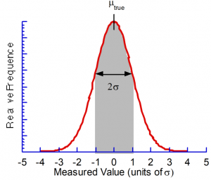
Now a few important things should be observed on this graph. First, the maximum is coincident with the “true value”, $\displaystyle {{\mu }_{{true}}}$ . Second, the curve is symmetric about $\displaystyle {{\mu }_{{true}}}$ , i.e. there are as many values higher than lower, as expected for a random distribution. Third, the width of the curve is related to the standard deviation, i.e. the larger $\displaystyle \sigma$ the larger the scatter in the data. Finally, the curve nears zero by $\displaystyle \pm 3\sigma$ away from $\displaystyle {{\mu }_{{true}}}$ , i.e. most experimental results are expected to lie within $\displaystyle \pm 3\sigma$ of the “true value.” This last fact enables quantitative conclusions to be drawn regarding the potential error in experimental data.

The area under the curve over specified intervals gives the probability of a given experimental value being within that interval of the true value. For instance, there is approximately 68% chance (∼2 out of 3) that an experimental datum will lie within $\displaystyle \pm 1\sigma$ of $\displaystyle {{\mu }_{{true}}}$ (the shaded area under the curve shown above), ∼95% chance (∼1 out of 20) for $\displaystyle \pm 2\sigma$ , and ∼99.7% chance (∼3 out of 1000) for $\displaystyle \pm 3\sigma$ . Further, if multiple measurements are taken and their mean is calculated, it can be shown that there is a 68% chance that any measurement $\displaystyle {\bar{x}}$ lies within the interval $\displaystyle \pm \frac{{1\sigma }}{{\sqrt{n}}}$ of the “true value” $\displaystyle \left( {{{\mu }_{{true}}}-\frac{{1\sigma }}{{\sqrt{n}}}\textless\bar{x}\textless\displaystyle {{\mu }_{{true}}}+\frac{{1\sigma }}{{\sqrt{n}}}} \right)$ where n is the number of measurements. The term $\displaystyle \pm \frac{{1\sigma }}{{\sqrt{n}}}$ is known as the standard error of the mean.

In fact, the problem can also be inverted. That is, given a mean, $\displaystyle {\bar{x}}$ , and a standard deviation, s, what is the probability that the “true value”, $\displaystyle {{{\mu }_{{true}}}}$ , is located within a specified interval. The naïve answer is that there is 68% chance that the “true value”, $\displaystyle {{{\mu }_{{true}}}}$ , lies within the interval $\displaystyle \pm 1s$ of any single measurement $\displaystyle x-{{s}_{{true}}}\textless{{\mu }_{{true}}}\textless\displaystyle x+{{s}_{{true}}}$ . This equation is correct if the true value of the standard deviation is known $\displaystyle s={{\sigma }_{{true}}}$ , but since $\displaystyle \sigma$ is determined from the experimental data, it too is subject to error (and can only be known after an infinite number of measurements).

Since $\displaystyle \sigma$ is also subject to error, additional uncertainty results, and for a finite number of measurements, $\displaystyle {\bar{x}}$ is not necessarily equal to $\displaystyle {{{\mu }_{{true}}}}$ and the calculated s is not necessarily equal to $\displaystyle {\sigma}_{{true}}$ . This problem was studied in the early 1900s by W. S. Gosset, a British chemist, who under the pen name, Student, established the following result for calculating confidence intervals:

$\displaystyle {{\mu }_{{true}}}=\bar{x}\pm t*\left[ {\frac{s}{{\sqrt{n}}}} \right]$

where t is known as Student’s t, and n is the number of independent experimental measurements. The value of t can be looked up in tables in statistics books, with some of the values given in the table below.

Degrees of Freedom (n-1)	Value of t for confidence interval of 95%	Value of t for confidence interval of 99%
1	12.71	63.66
2	4.30	9.92
4	2.78	4.60
5	2.57	4.03
100	1.98	2.63
$\displaystyle \infty$	1.96	2.58

It can be seen that for a large number like 100, the value of Student’s t approached that expected for the purely statistical ( $\displaystyle n=\infty$ ) case. [In Excel®, the t-value can be found using the function T.INV.2T(). For example, for (n-1)=4 degrees of freedom and 95% confidence, the Excel® formula T.INV.2T((1-0.95),4) would return 2.78 as given in the table above).

We are now prepared to interpret the titration results given earlier. Recall the result was 12.038±0.016 mL (n=5). We can now state that the “true value” has a 99% chance of being within $\displaystyle \pm 4.6\left( {\frac{{0.016mL}}{{\sqrt{5}}}} \right)=\pm 0.033mL$ of the mean, or $\displaystyle 12.01mL\textless \displaystyle {{\mu }_{{true}}}\textless \displaystyle 12.07mL$ . The fact that one is able to draw such rigorous conclusions even though the measurement is prone to some error is extremely useful. For instance, if you were to analyze Iowa City drinking water for atrazine and found 1.7 ppb (parts per billion by mass) using a technique with a standard deviation of $\displaystyle \sigma =\pm 0.14$ ppb and you only took two measurements, your result would be, $\displaystyle 1.7\pm 1.3$ ppb (to 95% confidence with n=2). In other words, to 95% confidence you could not say whether the pesticide level was above the government standard of 3 ppb, or even if there was any atrazine in the water at all. Yet with another measurement (n=3, and the same $\displaystyle {\bar{x}}$ and $\displaystyle \sigma$ ), you would obtain a result of $\displaystyle 1.7\pm 0.3$ ppb (n=3), and you would be able to say both that there was atrazine in the water and that its level was below the government standard.

Significant Figures

The general rule of significant figures is that the number of digits of a result presented should be consistent with the precision of the result. The standard deviation (or standard error of the mean) should be given to one significant figure and the mean value should match the decimal place of the standard error of the mean. So that the end result is not subject to cumulative round off error, at least one extra digit should be carried in intermediate calculations (thus 0.016 instead of 0.02 mL when the result will be used for a further calculation); round to one digit as the last step before reporting the result. Thus for reporting the mean of the example, $\displaystyle 12.038\pm \frac{{0.016\text{ mL}}}{{\sqrt{5}}}=12.038\pm 0.007\text{ mL}$ (n=5) would be acceptable, $\displaystyle 12.04\pm 0.03\text{ mL}$ (with 99% confidence, n=5) would also be acceptable.

Term	Symbol	Formulae	Excel® Function
Mean	$\displaystyle {\bar{x}}$	$\displaystyle \bar{x}=\frac{\sum_{i=1}^{i=n}{x_i}}{n}=\frac{x_1+x_2+\dots+x_n}{n}$	=average(A1:A5)
Standard Deviation	s	$\displaystyle s=\sqrt{\frac{\sum_{i=1}^{i=n}{(x_i-\bar{x})^2}}{n-1}}=\sqrt{\frac{\left(x_1-\bar{x}\right)^2+\left(x_2-\bar{x}\right)^2+\dots+\left(x_n-\bar{x}\right)^2}{n-1}}$	=stdev.s(A1:A5)
Number of trials	n
Student’s t		$\displaystyle {{\mu }_{{true}}}=\bar{x}\pm t*\left[ {\frac{s}{{\sqrt{n}}}} \right]$
Value of t at 95% confidence		Table	=T.INV.2T((1-0.95),(n-1))

References

Aikens, D. A.; Bailey, R. A.; Giachino, G. G.; Moore, J. A.; Tomkins, R. P. Integrated Experimental Chemistry, Vols. 1&2, Allyn and Bacon, Inc.: Boston, MA, 1978.
Miller, J. C. and Miller, J. N. Statistics for Analytical Chemistry, John Wiley & Sons: New York, NY, 1984.
Lide, D. R., Ed. CRC Handbook of Chemistry and Physics; CRC Press: Boca Raton, FL, 1994.

License

Icon for the Creative Commons Attribution-NonCommercial 4.0 International License

Significant Figures

References

License

Share This Book